LRP

Intro

The core concept behind the different LRP rules is the conservation property of relevance scores. By relevance score, we are referring to a measurement of how influential a particular input or a part of that input is to the output, which, in our case, is the Higgs likelihood prediction. We will define this properly later in this page.

Conservation Property

The conservation property for LRP is very much similar to the conservation law in physics. The wikipedia page of the latter states:

A particular measurable property of an isolated physical system does not change as the system evolves over time.

The conservation of relevance is very much the same: each layer of the model can be considered a closed system at different points in time. So, as relevance score propagates through a layer, the total amount of it stays the same.

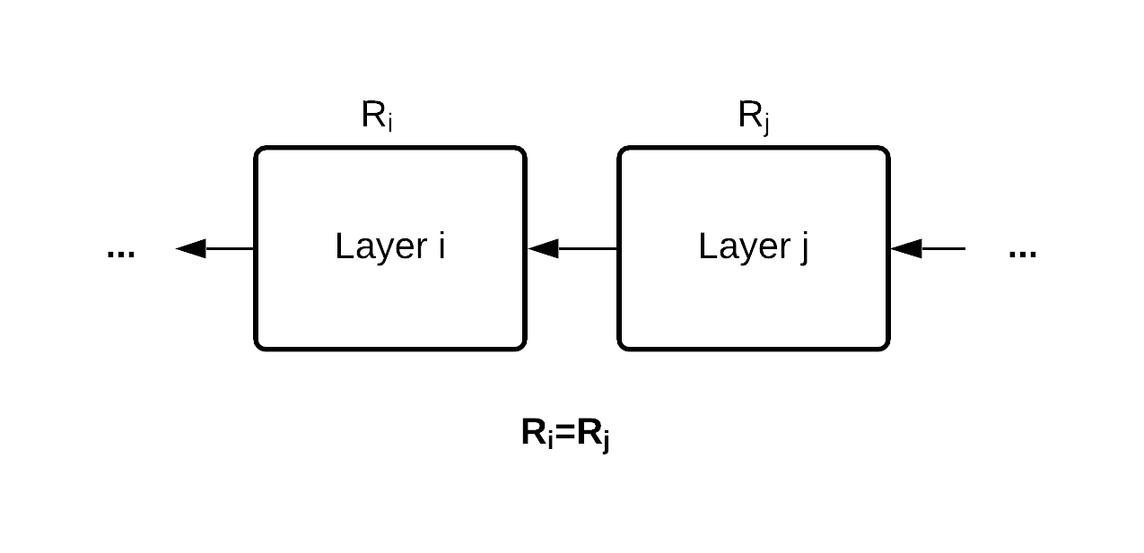
In our Higgs boson interaction network (HIN), things can get a bit more complicated. Other models have a more straightforward layer by layer architecture like in the plot above, whereas the HIN re-propagates certain layers, particularly the input and the input source node transformation, reapplying those values in multiple instances across the block layers. In simple terms, HIN reuses the input multiple times, and we have to adjust our LRP accordingly.

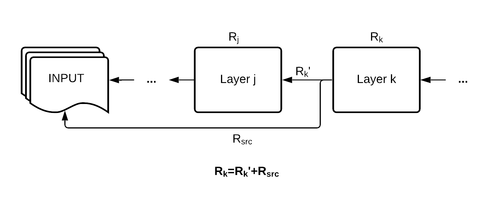
Remember the water and river analogy we made earlier? Like the flow of water in a river: the total amount of relevance score is conserved as it flows through the forks. Just like all the forks of the river eventually reaches the sea, the relevance scores propagates through the diverging paths, all reaching the input at the end from multiple points. Since the total amount of relevance score always stays constant, we could add up the relevance score attributed to a given layer and expect the same approximate value.

Now that we have an idea of how LRP propagates relevance scores through each layer, we can take a closer look at what happens within each layer.

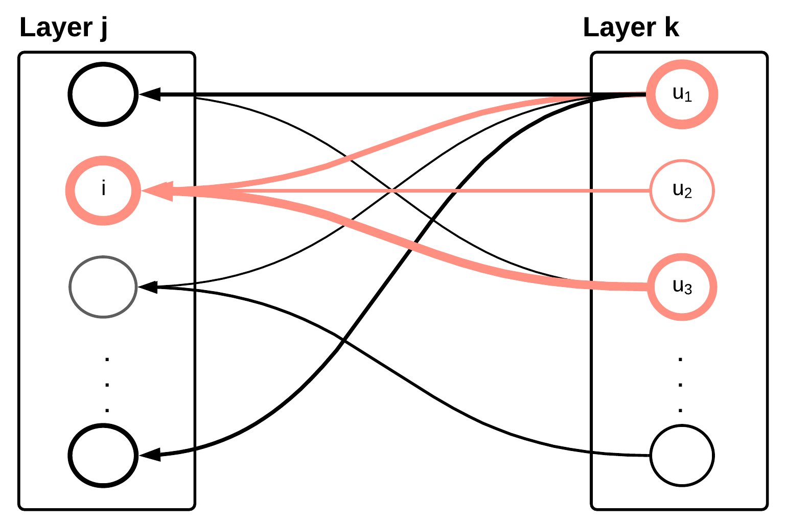
Within the layers, the same idea still applies, in a way similar to the relevance score propagating through the connections of consecutive layers. For neuron i in layer j,  it inherits a fraction of the relevance score from all neurons that it connects to in the consecutive layer k. The amount of relevance score neuron i obtains is decided by how much it has contributed to to those neurons that it connects to in layer k.

So how do we quantify neuron i’s contribution? It’s time to formally define what is the relevance score that we’ve been talking about.

Relevance score

Recall that we said the relevance score is meant to measure how much a particular part of the input has contributed to the output. So a natural way of quantifying it would be measuring how much change a particular input or a part of that input has induced on the output.

Consider the linear function below (some might recognize that this is in fact the definition of a linear layer in PyTorch):

Here x, y, and b are vectors, and W is a matrix.

Calculus tells us that the gradient of a function represents the rate of change per unit input. Since instead of unit input, we are more interested in the amount of change brought by a certain input, we actually take the product of the gradient and that input:

Naturally, the fraction of contribution for the u'th entry of input x would be the amount of change by this entry over the total change:

Now that we have the fraction of contribution, we can substitute it back into the equation to get the basic distribution rule of LRP, known as the LRP-0 rule.

In our project, we used a slightly more complicated distribution rule, the LRP-ε rule, for a better performance. The details of that are articulated in the main page.

Edge Significance Score

In the 3D network plots, we defined a new variable "edge significance" in order to measure how important each edge is to the prediction. This can be considered a variant of the relevance score.

The edges formed in the jet graphs are meant for the model to learn how each particle might have interacted with each other. They are not an actual part of the input but rather pathways that allow information to flow between the nodes. So if we consider each graph as a city and the edges are the roads that connect to each other, then intuitively the importance of each edge is decided by how busy it is, or the traffic passing through of it.

Following this idea, we defined the measurement edge significance to measure the importance of the edge by the amount of information, or contribution, flowing through it in the decision making process.

For an edge connecting from track t_i to track t_j, let's call it e_ij. Since each edge is defined by their source and destination nodes, the edge relevance of this edge is given by its source node and destination node, that is, it has 48 source node features and 48 destination node features.

The edge significance S_ij is a positive scalar value, given by the frobenius norm of the edge relevance score normalized with respect to all the edges in the graph. This is why those edge significance values in the chart do not have a negative denotation or threshold.